Rubix ML - Human Activity Recognizer

An example project that demonstrates the problem of human activity recognition (HAR) using mobile phone sensor data recorded from the internal inertial measurement unit (IMU). The training data are the human-annotated sensor readings of 30 volunteers while performing various tasks such as sitting, standing, walking, and laying down. Each sample contains a window of 561 features, however, we demonstrate that with a technique called random projection we can reduce the dimensionality without any loss in accuracy. The learner we'll train to accomplish this task is a Softmax Classifier which is the multiclass generalization of the binary classifier Logistic Regression.

Installation

Clone the project locally using Composer:

$ composer create-project rubix/har

Requirements

• PHP 8.3 or above

Recommended

• Tensor 4.1+ extension for faster training and inference

Tutorial

Introduction

The experiments have been carried out with a group of 30 volunteers within an age bracket of 19-48 years. Each person performed six activities (walking, walking up stairs, walking down stairs, sitting, standing, and laying) wearing a smartphone on their waist. Using its embedded accelerometer and gyroscope, 3-axial linear acceleration and 3-axial angular velocity were recorded at a constant rate of 50Hz. The sensor signals were pre-processed by applying noise filters and then sampled in fixed-width sliding windows of 2.56 seconds. Our objective is to build a classifier to recognize which activity a user is performing given some unseen data.

Note: The source code for this example can be found in the train.php file in project root.

Extracting the Data

The data are given to us in two NDJSON (newline delimited JSON) files inside the project root. One file contains the training samples and the other is for testing. We'll use the NDJSON extractor provided in Rubix ML to import the training data into a new Labeled dataset object. Since extractors are iterators, we can pass the extractor directly to the fromIterator() factory method.

use Rubix\ML\Datasets\Labeled;
use Rubix\ML\Extractors\NDJSON;

$dataset = Labeled::fromIterator(new NDJSON('train.ndjson'));

Dataset Preparation

In machine learning, dimensionality reduction is often employed to compress the input samples such that most or all of the information is preserved. By reducing the number of input features, we can speed up the training process. Random Projection is a computationally efficient unsupervised dimensionality reduction technique based on the Johnson-Lindenstrauss lemma which states that a set of points in a high-dimensional space can be embedded into a space of lower dimensionality in such a way that distances between the points are nearly preserved. To apply dimensionality reduction to the HAR dataset we'll use a Gaussian Random Projector as part of our pipeline. Gaussian Random Projector applies a randomized linear transformation sampled from a Gaussian distribution to the sample matrix. We'll set the target number of dimensions to 112 which is less than 20% of the original input dimensionality.

Lastly, we'll center and scale the dataset using Z Scale Standardizer such that the values of the features have 0 mean and unit variance. This last step will help the learner converge quicker during training.

We'll wrap these transformations in a Pipeline so that their fittings can be persisted along with the model.

Instantiating the Learner

Now, we'll turn our attention to setting the hyper-parameters of the learner. Softmax Classifier is a type of single layer neural network with a Softmax output layer. Training is done iteratively using Mini Batch Gradient Descent where at each epoch the model parameters take a step in the direction of the minimum of the error gradient produced by a user-defined cost function such as Cross Entropy.

The first hyper-parameter of Softmax Classifier is the batch size which controls the number of samples that are feed into the network at a time. The batch size trades off training speed for smoothness of the gradient estimate. A batch size of 256 works pretty well for this example so we'll choose that value but feel free to experiment with other settings of the batch size on your own.

The next hyper-parameter is the Gradient Descent optimizer and its associated learning rate schedule. The Momentum optimizer is an adaptive optimizer that adds a momentum force to every parameter update. Momentum helps to speed up training by traversing the gradient quicker. Instead of a raw learning rate, Momentum now accepts a Scheduler which supplies the step size for each batch. The Constant schedule outputs a fixed learning rate for the entire duration of training. A learning rate of 0.001 works well for this example so we'll leave it at that.

use Rubix\ML\PersistentModel;
use Rubix\ML\Transformers\PersistentTransformer;
use Rubix\ML\Transformers\Pipeline;
use Rubix\ML\Transformers\GaussianRandomProjector;
use Rubix\ML\Transformers\ZScaleStandardizer;
use Rubix\ML\Classifiers\SoftmaxClassifier;
use Rubix\ML\NeuralNet\Optimizers\Momentum;
use Rubix\ML\NeuralNet\Optimizers\Schedulers\Constant;
use Rubix\ML\Persisters\Filesystem;

$transformer = new PersistentTransformer(
    base: new Pipeline([
        new GaussianRandomProjector(112),
        new ZScaleStandardizer(),
    ]),
    persister: new Filesystem('transformer.rbx')
);

$estimator = new PersistentModel(
    base: new SoftmaxClassifier(
        batchSize: 256,
        optimizer: new Momentum(new Constant(0.001))
    ),
    persister: new Filesystem('model.rbx')
);

We'll wrap the transformer pipeline in a Persistent Transformer so it can be saved and loaded independently. The estimator is wrapped in a Persistent Model meta-estimator that adds the save() and load() methods to the base classifier. Both wrappers require a Persister object to tell them where to store the serialized data. The Filesystem persister saves and loads the data to a file located at a user-specified path in storage.

Setting a Logger

Since Softmax Classifier implements the Verbose interface, we can log training progress in real-time. To set a logger, pass in a PSR-3 compatible logger instance to the setLogger() method on the learner instance. The Screen logger that comes built-in with Rubix ML is a good default choice if you just need something simple to output to the console.

use Rubix\ML\Loggers\Screen;

$estimator->setLogger(new Screen());

Applying the Transformer and Splitting the Data

Before training, we apply the transformer pipeline to the dataset using the apply() method. This performs the Gaussian random projection and z-score standardization in-place on all samples.

$dataset->apply($transformer);

Next, we hold out a 10% validation slice of the data for monitoring generalization during training. The stratifiedSplit() method ensures each class is proportionally represented in both subsets. We pass the validation slice to the estimator via setValidationDataset() so that a validation score is reported at each epoch alongside the training loss.

[$training, $testing] = $dataset->randomize()->stratifiedSplit(0.9);

$estimator->setValidationDataset($testing);

Training

To start training the learner, call the train() method on the instance with the training dataset as an argument.

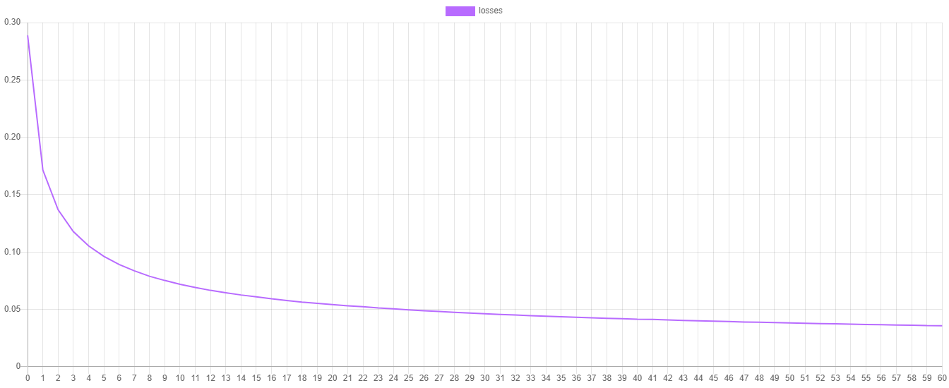
$estimator->train($training);

Training Loss

During training, the learner will record the training loss at each epoch which we can plot to visualize the training progress. The training loss is the value of the cost function at each epoch and can be interpretted as the amount of error left in the model after an update step. To return a table with the training progress at each epoch call the progress() method on the learner. Each row contains the epoch, the loss, and the validation score. Then we'll save the progress to a CSV file using the writable CSV extractor.

use Rubix\ML\Extractors\CSV;

$extractor = new CSV('progress.csv', true);

$extractor->export($estimator->progress(), overwrite: true);

This is an example of a line plot of the Cross Entropy cost function from a training session. As you can see, the model learns quickly during the early epochs with slower training nearing the final stage as the learner fine-tunes the model parameters.

Saving

Since we wrapped the transformer and estimator in their respective Persistent wrappers, we can save each by calling the save() method on their instances.

$transformer->save();

$estimator->save();

To run the training script, call it from the command line like this.

$ php train.php

Cross Validation

The authors of the dataset provide an additional 2,947 labeled testing samples that we'll use to test the model. We've held these samples out until now because we wanted to be able to test the model on samples it has never seen before. Start by extracting the testing samples and ground-truth labels from the test.ndjson file.

Note: The source code for this example can be found in the validate.php file in project root.

use Rubix\ML\Datasets\Labeled;
use Rubix\ML\Extractors\NDJSON;

$dataset = Labeled::fromIterator(new NDJSON('test.ndjson'));

Load Transformer and Model from Storage

To load the transformer and estimator we instantiated earlier, call the static load() method on the Persistent Transformer and Persistent Model classes with a Persister instance pointing to each artifact in storage.

use Rubix\ML\PersistentModel;
use Rubix\ML\Transformers\PersistentTransformer;
use Rubix\ML\Persisters\Filesystem;

$transformer = PersistentTransformer::load(new Filesystem('transformer.rbx'));

$estimator = PersistentModel::load(new Filesystem('model.rbx'));

Freeing Residual State

After loading the estimator, call the cleanup() method to release any leftover state from training. Since the model was persisted immediately after training, it retains state such as the optimizer's accumulated velocity which is no longer needed for inference. Calling cleanup() flushes this state and frees up memory.

$estimator->cleanup();

Making Predictions

Before making predictions, we apply the loaded transformer to the test dataset to project and standardize the features in the same way as training. Then we pass the transformed dataset to the predict() method on the estimator instance to obtain predictions.

$dataset->apply($transformer);

$predictions = $estimator->predict($dataset);

Generating the Report

A cross validation report gives detailed statistics about the performance of the model given the ground-truth labels. A Multiclass Breakdown report breaks down the performance of the model at the class level and outputs metrics such as accuracy, precision, recall, and more. A Confusion Matrix is a table that compares the predicted labels to their actual labels to show if the model is having a hard time predicting certain classes. We'll wrap both reports in an Aggregate Report so that we can generate both reports at the same time.

use Rubix\ML\CrossValidation\Reports\AggregateReport;
use Rubix\ML\CrossValidation\Reports\MulticlassBreakdown;
use Rubix\ML\CrossValidation\Reports\ConfusionMatrix;

$report = new AggregateReport([
    new MulticlassBreakdown(),
    new ConfusionMatrix(),
]);

Now, generate the report using the predictions and labels from the testing set. In addition, we'll echo the report to the console and save the results to a JSON file for reference later.

use Rubix\ML\Persisters\Filesystem;

$results = $report->generate($predictions, $dataset->labels());

echo $results;

$results->toJSON()->saveTo(new Filesystem('report.json'));

To execute the validation script, enter the following command at the command prompt.

$ php validate.php

The output of the report should look something like the output below. Nice work! As you can see, our estimator is about 97% accurate and has very good specificity and negative predictive value.

[
    {
        "overall": {
            "accuracy": 0.9674308943546821,
            "precision": 0.9063809316861989,
            "recall": 0.9048187793615003,
            "specificity": 0.9802554195397294,
            "negative_predictive_value": 0.9803712249716344,
            "false_discovery_rate": 0.09361906831380108,
            "miss_rate": 0.09518122063849947,
            "fall_out": 0.019744580460270538,
            "false_omission_rate": 0.01962877502836563,
            "f1_score": 0.905257137386163,
            "mcc": 0.8858111380161123,
            "informedness": 0.8850741989012301,
            "markedness": 0.8867521566578332,
            "true_positives": 2675,
            "true_negatives": 13375,
            "false_positives": 272,
            "false_negatives": 272,
            "cardinality": 2947
        },
    }
]

Next Steps

Now that you've completed this tutorial on classifying human activity using a Softmax Classifier, see if you can achieve better results by fine-tuning some of the hyper-parameters. See how much dimensionality reduction effects the final accuracy of the estimator by removing Gaussian Random Projector from the pipeline. Are there other dimensionality reduction techniques that work better?

Original Dataset

Contact: Jorge L. Reyes-Ortiz(1,2), Davide Anguita(1), Alessandro Ghio(1), Luca Oneto(1) and Xavier Parra(2) Institutions: 1 - Smartlab - Non-Linear Complex Systems Laboratory DITEN - University degli Studi di Genova, Genoa (I-16145), Italy. 2 - CETpD - Technical Research Centre for Dependency Care and Autonomous Living Polytechnic University of Catalonia (BarcelonaTech). Vilanova i la Geltrú (08800), Spain activityrecognition '@' smartlab.ws

References

• Davide Anguita, Alessandro Ghio, Luca Oneto, Xavier Parra and Jorge L. Reyes-Ortiz. A Public Domain Dataset for Human Activity Recognition Using Smartphones. 21th European Symposium on Artificial Neural Networks, Computational Intelligence and Machine Learning, ESANN 2013. Bruges, Belgium 24-26 April 2013.

License

The code is licensed MIT and the tutorial is licensed CC BY-NC 4.0.